1 Preface

Symmetry methods are taught universally in undergraduate inorganic classrooms, and have been for many years. Surprisingly, however, there are few resources available which cover the subject in deeper depth from a mathematical perspective, and of those, none are both accessible to undergraduates and detailed enough to provide a complete understanding. Some advanced texts exist from a mathematical or physics perspective, but the vast majority are heavily tailored towards advanced application (in the case of phyics) or highly abstract generalization (in the case of math), rendering them pretty much useless to nonexperts in those fields. A small number of advanced chemistry texts cover the subject - namely, Robert Carter’s Molecular Symmetry and Group Theory and F. Albert Cotton’s Chemical Applications of Group Theory each go into some detail - but both either fall short of a full-depth explanation (in the case of carter) or provide a significant amount of rigor, but don’t elaborate enough about the representation theory before jumping right into character theory, which in Cotton’s book left me particularly unsatisfied. Additionally, neither do a very thorough job of motivating the method physically, arguably the most important part of a grounded and satisfying explanation.

I personally think a thorough explanation and demonstration of the representation theory of molecules is a very useful exercise, even if actually applying the method without character theory becomes rather impractical to do by hand. Not only does it provide a strong foundation from which character theory builds upon, but it directly leads to some very interesting intuitive insights. So, my goal with this writeup is threefold: 1) lay out thoroughly and rigorously the representation theory of symmetry groups of molecules; 2) deeply motivate why understanding group and representation theory helps us approximate molecular orbitals efficiently; and 3) apply the method to several molecules, with detailed explanations and example matrices. These are the three aspects I was looking for when I first set out to understand this content, and I hope this could be the resource I was looking for.

However, this is probably not the resource that most chemistry students are looking for. While many mathematical insights can come from a rigorous approach with abstract tools, there’s a significant amount of visual intuition that also helps a great deal, and that’s something I can’t provide in text. However, I am also working on a youtube video made with Manim aimed at an audience with a less thorough mathematical background. I had originally intended that to be my SoME4 submission, but I was hit with the paradox of teaching: It’s harder and takes longer to write a shorter, simpler explanation than a longer, more rigorous one (”If I had had more time, I would have written a shorter letter” -CGP Grey). My goal is for that video to be as rigorous and satisfying as this writeup, albeit with some of the more involved (and less interesting) proofs left to this document, and it will focus much more on the visual and chemical intuition. That’s not to say that I won’t try to make this document intuitive - it’s just that I can’t guarantee groundbreaking revelations to anyone who doesn’t already have a very strong intuition via text alone about linear algebra and groups. (If you want to take a stab at it anyway, then hell yeah! I do really recommend 3blue1brown’s essence of linear algebra series ( https://www.youtube.com/playlist?list=PLZHQObOWTQDPD3MizzM2xVFitgF8hE\_ab) as an introduction to the visual intuition of linear algebra, which has been indispensable for me in my research and in writing this video).

Okay, last thing before I shut up and start talking: I won’t be covering character theory in detail here. As I mentioned before, using character tables to find multiplicity of irreducible representations is a very useful trick, and when combined with projection to extract basis vectors, it can fully skip the need to do decomposition manually; however, all explanations of it (as they exist online, which is nearly as rare) are necessarily rooted in the theory presented here, so to understand them, it’s critical to understand representation theory and invariant subspaces. If all goes to plan, I do intend to make a follow up video + article about character theory and the projection operator method. For now, I explain at the very end exactly what character theory does in the context of representation theory, and briefly outline the projection operator method (just to get it written down) and its role in completing the shortcut.

2 Introduction: Symmetry, Group Theory, and Molecules

The fundamental problem we will be tackling today is very simple to describe: You have a molecule. You know its atoms and structure, but you want to know its bonds. More specifically, you want to know the energy and shape of the various orbitals its electrons can occupy. In other words, you want its molecular orbitals: the wavefunction describing the position of an electron associated with each electronic state.

You already know how to do this for atoms - either because they had you derive it in a physics or physical chemistry class, or simply because you’ve seen them every time you enter a chemistry class: s orbitals, p orbitals, d orbitals, etc, each parameterized by shell and angular momentum. Although atomic number affects the magnitude of the nucleus’ pull on its resident electrons, the shapes are all in the family of hydrogen-like orbitals: the first electronic wavefunctions to be solved analytically in closed form in the 1920s¹ .

In fact, they were the only wavefunctions to be solved in closed form. They still are. It turns out having multiple nuclei tugging on electron clouds is too much for the tools of modern differential calculus to handle; in fact, the hydrogen orbitals can’t even be symbolically solved when there is more than one electron around the molecule for the same reason.

This leaves us in a bit of a predicament with our molecular orbital task. If we can’t solve the equations that are supposed to produce the orbitals, how can we ever be expected to find them?

The answer is twofold. We will, at the end of the day, be using an approximation which lets us turn the problem into something more tractable. More interestingly, however, we will be searching for the orbitals by determining properties we know they must have, and then guiding our search accordingly. And for that, we will be using molecular symmetry.

3 Molecular Symmetry

For the sake of time, I will be assuming you know the basics of molecular geometry and molecular symmetry. There are many clear and concise resources on Google and YouTube that walk one through the various symmetry operations and assigning point-groups to molecules. I will, however, talk briefly about why we care about symmetry.

Each molecule has a particular arrangement of atoms which defines its geometry. Since we are only going to be solving for single-electron orbitals (because Fock knows that’s hard enough² on its own), we can assume that the electric force/potential field which will determine the shapes of our orbitals is influenced solely by the positions (and nuclear charge) of each atomic nucleus. Thus, for any given molecule, there will very often be some number of rearrangements of the atoms which will leave the electric potential - and thus the molecular orbitals - entirely unchanged. These rearrangements are known as the symmetries of our molecule, and, taken as a whole, the set of a molecule’s symmetries form a mathematical group (whose group action is the act of composing symmetry actions, e.g. performing one action, then the other).

While it might not seem like a big deal, these actions rigorously encode a set of equalities we can use to characterize the potential field and thus the orbitals generated by it. Since we generally only consider the symmetry actions which can be described as transformations of space - reflections, rotations, and inversions - we can consider the effect of a symmetry action on any object in the molecule’s 3d space. Notably, if we consider the chemical environment of a particular wavefunction - that is, the potential around it and the forces thus imparted that would change the shape of the wavefunction over time - we know it must be the same as the chemical environment of any wavefunction symmetrical to the first, such that applying a symmetry to the first can produce the second.

This means that if two wavefunctions are symmetrical to each other, they must exist in the same chemical environment as each other, and therefore, they will both evolve symmetrically to each other over time. Since the stable molecular orbitals of a molecule are those which don’t change over time³ , that means if two wavefunctions are symmetrical to each other, and one of them is a molecular orbital, the other is a molecular orbital as well. And remember, ”symmetrical to each other” means there exists a symmetry action which brings one to the other - so if you have a molecular orbital (MO), then all of the wavefunctions you can get by applying the symmetries of the molecule to that MO will also be MOs. Additionally, since the energy of an orbital is a property of its shape in the potential well, all of those equivalent MOs will have the same definite energy as the first.

What this tells us is that space of all possible wavefunctions can be grouped into symmetric sets, and that our molecular orbitals will always be grouped with other identical MOs. What the remainder of this writeup will document is how we can classify these symmetric sets - and the linear spaces they form - both by their size and by the action of the group upon them. I will then show that by grouping together these symmetric spaces by their classification, and by finding a basis for these groupings using the atomic orbitals of our atoms, we can greatly simplify the process of determining our molecular orbitals.

4 Orbits and Invariant Subspaces

In the field of group theory, these ”symmetric sets” are known as orbits. Specifically, if a group G describes a set of actions on a set, in this case the set of wavefunctions, then the orbit under G (written orbit_G) some element Ψ of that set is defined as {g ∗ Ψ|g ∈ G} - that is, the result of applying g to Ψ for each action g in G.

It’s important to note that, although every element will have its own orbit, not all orbits are equivalent. For example, some orbits will be different sizes; some objects might be totally symmetric with respect to the group, so that every symmetry action maps that element to itself. In that case, the orbit would only be a single element! On the flipside, some elements might be totally asymmetric, so that every symmetry action will result in a different element. Other orbits might be the same size as each other but be the result of the group acting differently on the seed element - for example, one seed element might be totally symmetric under reflection, but not rotation, while the other seed element is totally symmetric under rotation, but not reflection. This inherent structure to how the group acts on an orbit is what we’re interested in describing, for reasons that will be made clear in the next section.

However, describing the action of the group on each orbital is a very complicated task, and for a general group, doesn’t actually help us that much. But this is no general group! Remember, we defined our symmetry group to be composed solely of transformations of space. This means that the action of our group on the space of wavefunctions can be described linearly.⁴

This opens up the door to many possibilities. First, it means that we can describe the group action with matrices, which computationally opens the door to a huge number of possibilities that linear algebra provides. Secondly, it allows us to relate the various orbits-of-wavefunctions to each other by way of these matrices. We will address both of these using invariant subspaces. I’m assuming you have a decent background in linear algebra, but as a brief reminder, a subspace of some larger vector space V is a subset of V in which addition and scalar multiplication are closed. You can think of it as some n-dimensional ”slice” of V - for example, an (infinite) line, an (infinite) plane, and the point at the origin are all subspaces of V - 1, 2, and 0 dimensional subspaces, respectively. For a subspace to be invariant under a linear action - or in our case, a set of them - means that every vector in that space gets mapped to another vector in that space under the action (or under all actions in the set). In other words, each action reorganizes the vectors in the subspace - rotating, reflecting, or otherwise transforming them - but does not move any vectors out of (nor, because group actions are always invertible, into) the space.

Invariant subspaces are very useful when trying to understand a (set of) linear action(s), because any linear action can be represented on a (finite) invariant subspace as matrix. Specifically, given a basis b₁,b₂,... of vectors in that subspace, each element of the matrix representation of a linear action g can be defined as a_ij = b_i ⋅ g ∗ b_j. It’s important that the subspace be invariant so that g ∗ b_j can always be expressed as a linear combination of your basis! For a given invariant subspace (and basis), the set of matrices corresponding to each linear action of the group is known as a representation of the group on that space⁵ . Although the actual entries in each matrix are dependent on the particular basis, we often like to talk generally about the group’s action on the space as a whole independent of the basis. To that end, we usually call two representations of a group the same if one can be transformed into the other by a change-of-basis - algebraically, if for each matrix A_i from the first representation, the corresponding matrix in the second can be described as MA_iM⁻¹, using the same change-of-basis matrix M for each element in the representation. Thus, up to this notion of equivalence, every invariant subspace can be classified by the representation of the group on that subspace, which describes how that subspace is linearly transformed by the different actions of the group.

Critically, the span of the orbit of a vector is always an invariant subspace. Recall that the span of a set of vectors is the set of all possible linear combinations of those vectors, and is always a valid subspace. Lets say the orbit of a vector v₁ is {v₁,v₂,...}, and will call the subspace V = span{v₁,v₂,...}. Then each element in the subspace can be described as v = c₁v₁ + c₂v₂ + .... The subspace V is invariant under G iff, for every vector v in V , g ∗ v ∈ V for every g ∈ G. g ∗ v = g ∗ (c₁v₁ + c₂v₂ + ...) = c₁g(v₁) + c₂g(v₂) + ... by linearity of g. Note that the orbit itself must be invariant under G, as if some element v_i ∈ orbit_G(v) = g ∗ v, then h ∗ v_i = h ∗ (g ∗ v) = (h ∗ g) ∗ v; since h ∗ g ∈ G, (h ∗ g) ∗ v ∈ orbit_G(v). Thus, g ∗ v_i ∈ V , meaning g ∗ v is some linear combination of vectors in V - which by the definition of a subspace, means g ∗ v ∈ V . Thus, the span of an orbit of a vector forms an invariant subspace.

With these two tools, we can return to our original goal of classifying the symmetric sets of our wavefunctions, by extending that to classifying the symmetric spaces of wavefunctions and using those classifications to compute the value of our molecular orbitals.

5 Invariant Subspaces of MOs

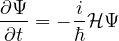
Earlier I mentioned that we know that molecular orbitals come in symmetric sets because the chemical potential of the molecule is symmetrical. While this is true, it pays to be a little rigorous, so let’s look a little deeper at the physics. At the core of wavefunction evolution is a linear operator known as the Hamiltonian, ℋ. When I say at the core, I’m being quite literal: it is the fundamental component of the Schrödinger equation, which describes how any wavefunction Ψ evolves over time.

(1)

When we talk about atomic or molecular orbitals (of an atom or molecule respectively), what we mean are the solutions to this equation which describe the quantum state of an electron. Specifically, we want the time-independent solutions to this equation, meaning that Ψ doesn’t observably change over time. ”Observably” is a loaded word there which has implications beyond the scope of this document, but essentially the requirement is that the probability density function describing an electron’s state doesn’t change. The probability density is the magnitude of the wavefunction squared; since a wavefunction is complex, this means that the wavefunction is allowed to change in phase over time, but not in magnitude. Specifically (and this is where the nuances of observability come in), to be time-independent, the wavefunction is allowed to globally change phase over time - that is, its value at every point must change phase at the same rate - but there must be no changes in magnitude or global phase.

That’s a very complicated requirement, but luckily it has a simple(r) solution: must be a 90°or -90°phase-offset scalar multiple of Ψ. To realize why, imagine Ψ evaluated a single point x, somewhere in the complex plane. If we want to add some value which will infinitesimally rotate Ψ(x) around the origin, the complex number we add must be perpendicular to Ψ such as to not change its distance to the origin. So long as our dΨ always remains perpendicular as Ψ changes, it will travel in a smooth circle. Since the effect of this rotation depends on the radius to the origin, it’s important that the magnitude of our added vector scales with the magnitude of Ψ at every point, so that all of Ψ is rotated at the same rate.

Hopefully that description was illustrative, but if not, fear not: we are at its end. We know that must equal Ψ, rotated 90°and potentially multiplied by some real number; since ℏ is just a real physical constant, and multiplying by i rotates complex numbers by 90°in phase, we know that ℋΨ = λΨ for some real number λ. This equation is often known as the time-independent Schrödinger equation, as it can be used to calculate all of the time-dependent solutions to the Schrödinger equation.

Those familiar with linear algebra will recognize this as an eigenvector equation. An eigenvector of a linear operator A is any vector x such that Ax = λx for some scalar λ; the value of λ corresponding to a certain eigenvector x is known as the corresponding engenvalue. It turns out the eigenvalues of the Schrödinger equation - the eigenvalues of the Hamiltonian operator - are also very important; they represent the corresponding energy of an orbital. That’s why in most physics texts, you’ll see the above equation written ℋΨ = EΨ.

Thus, by finding solutions to the time-independent Schrödinger equation, we compute both the orbital and its energy. How cool is that! However, though eigenvector-eigenvalue problems are arguably the most fundamental class of computational problems in linear algebra, solving them numericalls is often extremely computationally costly. In this case, especially, it’s quite expensive, as evaluating ℋΨ a single time requires a complex 3d integral of the wavefunction and the potential field over all of space. It should be clear doing any of that by hand is completely out of the question. The ultimate goal of the symmetry approach, therefore is to make this process as easy as possible - in some cases, making the act of finding solutions not only possible to do by hand, but intuitive.

To do so, we return to symmetry. When we say that the evolution of an orbital is the same as its symmetric counterparts, we are precisely talking about the Hamiltonian: That if one were to move an orbital to a symmetric location, evolve it, and then move it back, the the result would be the same as if you just evolved it in place. Because the Hamiltonian rigorously describes this evolution, we say that for any action g in G, g ∘ℋ∘ g⁻¹ = ℋ, or just g ∘ℋ = ℋ∘ g. In other words, for any wavefunction Ψ, ℋ(g ∗ Ψ) = g ∗ (ℋΨ).

This has a very interesting property for our eigenvectors in particular - since ℋΨ = EΨ, ℋ(g ∗ Ψ) = g ∗ (ℋΨ) = g ∗ (EΨ). Since the action of g is linear, g ∗ (EΨ) = E(g ∗ Ψ), so ℋ(g ∗ Ψ) = E(g ∗ Ψ) - so if Ψ is an eigenvector with eigenvalue E, then so is g ∗ Ψ! This precisely matches our intuition from before, but it gives us an extra tool, because the set of eigenvectors with the same eigenvalue (which are known as degenerate eigenvectors) have a very important property: they form a complete subspace. Specifically, if we have eigenvectors v₁ and v₂ of an operator A, where Av₁ = λv₁ and Av₂ = λv₂, then for any linear combination c₁v₁ + c₂v₂, A(c₁v₁ + c₂v₂) = c₁A(v₁) + c₂A(v₂) = c₁λv₁ + c₂λv₂ = λ(c₁v₁ + c₂v₂). In other words, any linear combination of eigenvectors of the same eigenvalue is also a degenerate eigenvector with that eigenvalue.

What this means is the span of the orbit of our eigenvectors - which, remember, is an invariant subspace under G - is an invariant subspace entirely composed of degenerate eigenvectors. This helps us in two ways: 1) we can classify it by the representation of G upon it, and 2) we no longer need to worry about finding a specific set of symmetric molecular orbitals - all we need to do is find a subspace of them, and we can pick any set we like from within it.

Of course, that’s still a daunting task. But now that we know that we’re looking for invariant subspaces, there’s a final tool that will tie everything together.

6 Irreducible Representations

One aspect I didn’t mention earlier is the concept of the decomposition, otherwise known as reduction⁶ of a space into invariant subspaces. By decomposing, I mean finding a collection of invariant subspaces which, together, reconstitute the whole space; for example, the xy plane and the z axis together constitute euclidean 3d space, as any vector in 3d space can be described as a linear combination of a vector from the xy plane and a vector parallel to the z axis. This joining of subspaces is known as the direct sum; while I won’t go into detail here, it may be useful to look up the details if you aren’t familiar. What’s most important is that the subspaces be jointly linearly independent; that is, no vector in one can be written as a linear combination of vectors from any other. This allows us to say that the dimensionality of the whole space is the sum of the dimensions of each individual subspace, and we can find a basis of the whole space by joining bases from each individual space.

An invariant subspace is therefore decomposable, or reducible, if it itself contains linearly-independent invariant subspaces (besides itself and the trivial space 0) which constitue the space (via the direct sum). A reducible invariant subspace can then be broken down into strictly smaller subspaces. On the flipside, an invariant subspace indecomposable, or irreducible, if it cannot be broken down in this way. All one dimensional invariant spaces are irreducible, as it has no subspaces other than itself and the trivial space; however, there exist higher dimensional ones. We can similarly name the representations of these spaces as reducible or irreducible, as indeed, the information of whether a space has invariant subspaces is precisely dependent on how the representation upon it transforms its vectors.

Irreducible representations are fantastically useful. For one thing, finite groups have finitely many of them (as usual, under similarity by change-of-basis). That means, no matter how large your space is, the irreducible representations will only ever be one of the finitely many that correspond to the group. Additionally, a very famous theorem - Matchke’s theorem, for which there are many proofs online, so I won’t give one here - states that any invariant subspace can be decomposed into a complete set of irreducible representations of a finite group, and, moreover, that the representations in that decomposition is unique; that is, no matter what subspaces you decompose the larger space into, the number of each irreducible representation in the final decomposition will be the same.

With this decomposition tool in hand, we can finally, finally, lay out our primary claim about the eigenvectors of the Hamiltonian: Given a subspace of wavefunctions V on which the hamiltonian is invariant, a full basis of eigenvectors can be found in irreducible representations of V .

Why is this true? Because the spaces of degenerate eigenvectors are invariant under the group! Even if they are reducible⁷, they can always be decomposed into irreducible subspaces which are entirely composed of eigenvectors with the same eigenvalue. Because eigenvectors with different eigenvalues are always linearly independent, there is a set of these irreducible subspaces composed of eigenvectors which reconstitute the whole set of wavefunctions V - in other words, they are a valid decomposition of the group into irreducible invariant subspaces. y Matchke’s theorem, that means any irreducible decomposition of V will consist of the same number of subspaces of the same representation as our eigenvector decomposition.

Note, however, that this doesn’t guarantee that the spaces themselves must be the same. In a space composed of a pair of irreducible subspaces with the same representation, you can actually find an infinite number of decompositions into other pairs of irreducible subspaces with that same representation.

Even still, we can get most of the way there, because of one very important proof: If a vector v is a nonzero sum of vectors from irreducible subspaces with different representations, the vector does not belong to any irreducible subspace. The proof brings together everything we’ve learned thus far, so buckle in. Say we have two irreducibly invariant subspaces X and Y . Each induces a representation of G; let A_g the representation of g on X for all g ∈ G, and similarly B_g is the representation of g on Y for all g ∈ G. Take any vectors x and y from X and Y respectively, both x and y nonzero; then z = x + y is not a member of an irreducibly invariant subspace. Recall from before that span(orbit_G(z)) is an invariant subspace; in fact, it is the smallest invariant subspace to which x belongs, as any invariant subspace containing z must also contain orbit_G(z) by definition. Let Z = span(orbit_G(z)). Claim: Z is reducible; specifically, Z = X ⊕ Y . First, every vector in Z is a sum of vectors from X and Y , as g ∗z = g ∗x + g ∗y; since X and Y are invariant, g ∗x ∈ X and g ∗Y ∈ Y . Since Z is the span of all elements g ∗ z for each g ∈ G, each element in Z is therefore a sum of vectors in X and vectors in Y . Thus, Z ⊆ X ⊕ Y . By matchke’s theorem, this means Z must have the same representation as either X, Y , 0, or X ⊕ Y . We know dimZ > 0, since we assume X and Y nontrivial; the question remains whether Z has the same representation as either X or Y .

Thus, our problem reaches its final form: Determine which irreducible subspaces house the eigenvectors of the Hamiltonian. The process for this is relatively straightforward: Find a complete decomposition of our space into irreducible representations, combine the subspaces with the same representation via the direct product, and then find a basis of eigenvectors in each smaller space. Since we know we can find a complete basis of eigenvectors in our irreducible spaces, and since we know that for each irreducible representation, every subspace inducing that representation of G can be found as a subspace of the direct product of enough spaces with that representation, we know that each collection of irreducible spaces will contain all of the degenerate spaces of eigenvectors belonging to that representation.

7 Wrapping Up

Actually applying this to molecules is another matter. Despite what it might seem from the density and complexity of this text, however, the process is not all that hard to understand visually. It’s really only a select handful of proofs that necessitated the existence of this document, and even then, part of me still wonders if all of these have some clever visual or intuitive explanation that could cut the text’s length in half. Briefly, the molecular approach goes as follows:

1 Pick a finite basis of orbitals on which to work

1a) Usually this will be a selection of the atomic orbitals of each atom, though for computational approaches these ”atomic orbitals” are often arbitrary localized wavefunctions which don’t actually match the atomic s, p, d, etc orbitals at all

1b) There are only two important requirements for the basis:

1b)1. It must be invariant under the group - this one’s pretty easy to satisfy, as you just need to make sure you include the orbit-wavefunctions of every function you include. E.g. if you include one hydrogen’s s orbital in ammonia, you need to include the other two.

1c) It must be invariant under the Hamiltonian. This one is basically impossible - since we know that in the broader molecule, any space with the right symmetry is going to interact with our chosen subspace. By picking appropriately-energied atomic orbitals, we can greatly reduce the error from restricting ourselves to a finite basis, but there’s not a lot we can say conclusively.

2 Find irreducible subspaces in that basis

2a) This is the process of labeling orbitals by their symmetry and finding SALCs. The video will cover this process in significantly more detail, as it is often unsatisfyingly skipped using character theory.

3 Construct the combined irreducible representation spaces by grouping the irreducible subspaces by representation

4 Represent the Hamiltonian numerically on each of the combined spaces

5 Solve each represented Hamiltonian for the eigenvector basis of that irreducible representation

Finally, to connect this to character theory: Character tables store information about the various irreducible representations of a finite group. Specifically, each element in the table represents the trace of the corresponding matrix used to represent G. Since we say two representations are equivalent if they are related by a change-of-basis, and the trace doesn’t change under change-of-basis, the trace description in a character table is consistent with any representation. Moreover, for reasons that currently bewilder me, the rows of a character table - that is, the sets of traces corresponding to each element of the group (column) from each irreducible representation (row) form an orthogonal vector basis for the space of all representations. Thus, given the representation of G on some reducible subspace, taking a (modified) dot product between the set of traces of that representation and the various rows of the character table can tell you what irreducible representations span the space while knowing almost nothing about the space.

This becomes incredibly useful with the Projection Operator, which allows you to, given a target irreducible representation, project any vector into that set of all subspaces with that representation. Since character tables gives us a way to know the irreducible representations without doing any actual decomposition, and the projection operator method lets us project into those irreducible representations and thus gives an easy way to find (a) basis, together they skip a massive chunk of the work one would do to decompose these spaces by hand. In the next video and writeup, I’ll talk about how and why this works.

Well, that was quite a doozy - but of course, as Huckleberry Finn famously said, ”If I’d have had more time, I would’ve written a shorter letter”. I hope this helps someone feel better at least; and if not, it’ll serve as a nice personal reference guide. Thank you so, so, much for reading, and if you got here without help from the Summer of Math Exposition and 3blue1brown, you should go check them out! #SoME4 has so many good submissions this year, and most of them aren’t even out when I’m writing this! Let’s keep math edutainment youtube alive and strong.